An Enigma: Transmission Of Epidemic Influenza (part 13)

Today I use ARIMA techniques to explore the percentage of influenza to all cause deaths for males over the period 1920 - 2022

Jul 04, 2025

If you are reading this you didn’t run fast enough!

I guess we better start with a slide of what I am going to try and model. Here it is…

There we are; no less than 9 time series indicating the rise and fall of the percentage of influenza to all cause death for males over the period 1920 – 2022. It’s worth contemplating this for a while for there are several curious features. First up, for my money, is the sudden return of influenza as a nasty in 2001. Those who have followed this series from the outset will already have realised this coincides with a coding change following a WHO ruling on death certification (yep, it’s that rule 3 curve ball coming back at us). This ruling and its implementation by ONS serves to amplify the situation very much like turning up the gain on your guitar amp. In effect we are looking at a hybrid dataset with the pre-2001 data not being of the same ilk. Ideally we’d chop this monstrosity into two sensible slices but I’d like to start out tackling the beast as it is, for as sure as eggs is eggs the authorities are going to milk the situation. Add a bit of flour and we have a batter!

We can make a start by sticking a piece of buttered baking parchment over the period 2001 – 2022 and looking at what we’ve got left by way of a coherent series. A decline indeed, and not just a wimpy decline neither but a handsome decline into virtual nothingness: surely this can’t be good for business! Some with vested interests may try and palm this benefit off onto the annual flu jab programme but those with eyes will see this decline was already trundling before the flu vaccine was even developed, let alone distributed to the masses.

In the early days we observe a fair few green spikes that indicate a preponderance of males aged 35 - 44 and 45 – 54 years. Curious. I’m not buying into the notion of a sex-specific pathogen so something else must have been going on that we’re not being told about. Quite why this anomaly wasn’t flagged up decades ago is beyond me. Another feature are those two whopping great spikes for young males aged 5 – 14 and 15 - 24 years centred on 1957. Whilst some may try to argue that this is a singularly peculiar sex- and age-specific pathogen at work my money is on something more like the after effects of a vaccination campaign or unfortunate choice of treatment for kiddies that nobody wants to talk about these days.

Move that buttered baking parchment to the left and we see the same anomalies poking up again in the new, and rather amplified age of the hyper-flu coding mess. Yep, it’s those same blue spikes indicating a peculiar and repetitive vulnerability among young males. The exception is that super-sized orange spike for males aged 65 – 74 years for 2016, and my money is again on something the establishment is doing rather than a bug. Whether or not the establishment realises this is a different matter! That may sound like an odd statement to make but then again I spent 8 years helping consultant cardiac firms get to grips with clinical effectiveness and long term outcomes rather than living in the surgical moment.

Let us now see what ARIMA makes of this when run in expert mode…

The Eyes Of ARIMA

Before we do this it might be prudent for us to look through the same eyes as the ARIMA procedure. By that I mean the algorithm employed will want to make the time series stationary, and to do that it’ll take the first order differential to yield year-on-year changes, thereby removing any trend. It will then employ a natural log or square root transform to iron out some of that heteroscedasticity (changing variance over time). This is what the data will look like after these two transformations:

Different innit? I’ll say!

Gone are those early spikes, including the 1957 whopper and, instead, we have a rather spiky looking recent past. Being a differential series we should note that each upward spike will be accompanied by a following downward spike, with the grand mean of each series centred on a zero percent change. The compression afforded by the natural log transform serves to make all the spikes the same height or as near as dammit. This is what a stationary series looks like and this is what the ARIMA procedure will model because it is looking for periodic behaviour. Please bear this distinction in mind for, as suspicious humans, we’ll be scanning the data for spikes and trends and not periodicity!

Even with this statistical googly bowled at us we should be able to cogitate effectively after another cuppa. For example, my eyeballs have alerted me to a preponderance of deep blue spikes from 1975 onward. This tells us that something particularly odd has been going on with regard to young males aged 5 – 14 years; and we should expect to see this reflected in a long list of outlying years. If this is indeed the case we might start asking why this age group is constantly clobbered over time. No doubt some of you will make the leap to junior and senior school vaccination schedules, but let’s get to see some tables first…

ARIMA Models

Now is the time to go into the kitchen and make a cup of tea if you are of a nervous statistical disposition for I am about to unleash monstrous tables…

Deep breaths, deep breaths!

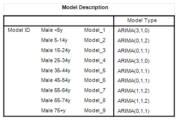
Model Description

If we start with the small table titled ‘Model Description’ we get to see the range of model structures adopted of the form ARIMA(p,d,q) where ‘p’ is the order of the autoregressive component (AR), ‘d’ is the order of differencing and q is the order of the moving average term (MA). All exhibit d=1, as we may expect, for all nine time series plummet over time and this needs addressing (a.k.a. being transformed into a stationary process). Beyond this we have a smatter of autoregressive and moving average components of order 3 and less. ‘Order 3’ in this instance means 3 years, so for males aged under 5 years and males aged 25 – 34 years there is a 3-year effect whereby what was happening 3 years ago can be used to predict what might be happening in the current year. I call this the ‘memory effect’ and it’s a rather strange concept to apply to what is supposed to be a highly dynamic constantly mutating pathogen. Far easier to think in terms of medical thinking IMHO... or even fashions in death certification!

Model Statistics

Moving down to the table titled ‘Model Statistics’ what I want folk to take away here are the reasonable model goodness-of-fit statistics that hover between 0.394 and 0.779 in terms of stationary R-square1. In plain English ARIMA made a good go of it. One column that proves to be mighty interesting is the count for the number of outlying years. Leading the way is males aged 5 -14 years with 7 notable outlying years, and we might like to cogitate on what makes this group particularly vulnerable. As a betting man I’d have put money on males under 5 years and males aged 75 years and over as being the most vulnerable to a pathogen; but perhaps we are looking at clinical rather than physiological vulnerability, the word being iatrogenic. There is additional food for thought on the table if we consider when we start jabbing kids in earnest.

ARIMA Model Parameters

And so on to the ARIMA Model Parameters whopper. Bizarre as it may seem there isn’t anything as decidedly juicy in this table, it being a rather boring summary of model coefficients. My favourite aspect is the column that would be full of the phrase ‘Natural Logarithm’ were it not for the square root transformation applied to the male 25 - 34 year time series. This tells us that this series has a slightly different overall shape.

Outliers

Arguably the juiciest table is the final table of detected outliers. My eyeballs dived straight in to the 7 outliers for males aged 5 – 14 years to discover all is not a tale of woe and neglect, for there are no less than 4 negative coefficients. What we can say, therefore, is that this is a particularly volatile age group.

According experts 2020 and 2021 are years when the flu disappeared from the face of the Earth – coz COVID. Well, according to this table, this only holds true for males aged 5 – 14 years, who exhibit a negative coefficient of -5.610 for 2021 (p<0.001). No other group shows any sign of a sudden decline when it comes to influenzal death as a percentage of all cause death. Curious!

In terms of bad flu years our eyeballs should be weeding out 1988, 1989 and 1999 for males aged 5 – 14 years, 2001 for males aged 15 – 24, 45 – 54 and 55 - 64 years, 2002 for males aged 35 – 44 years, 2003 for males aged 65 – 74 years, 2012 for males aged 65 – 74 years, 2014 for males aged 15 – 24, 35 – 44 and 75+ years, 2016 for males aged 65 – 74 years, 2017 for males aged 55 – 44 years, and 2018 for males aged 75+ years. This is a rather strange set of incidents. Aside from the 5 – 14 year group nothing is showing before 2001, and even with the volatile 5 – 14 year group nothing is showing before 1988.

Could It Be Coding?

Barry Manilow once asked if it could be magic… and I’m now asking if it could be coding. If it is coding then we are in a fine analytical pickle, and make no mistake. At this rate I might have to get my cleaver out and model just 1920 – 2000, for the period 2001 – 2022 is far too short to throw into ARIMA alone. Dangnabit!

I’ll tell you what, though, we can take those outliers detected for 2001 – 2022 and ask if they make biological sense. To my mind they don’t make any sense if I try and pin them to the spread of a mutating bug within a population and over time. They only start to make sense to me if I assume coding nonsense and/or iatrogenic death is at play. With that I wild notion thrown on the table I guess we better stop there and have a breather…

Kettle On!

Not to be confused with common or garden R-square which ain’t the same thing.

Discussion about this post

Chris Marmont

Jul 7

Thank-you for this fascinating series and all your previous writings.

With respect to your comment, “… my money is again on something the establishment is doing rather than a bug”, here’s one idea of possible establishment involvement. I hope this is not too off-the-wall.

After a couple of years of recommendations from Dr. Tess Lawrie and her colleagues at World Council for Health, I bought and am currently reading The Invisible Rainbow, A History of Electricity and Life, by Arthur Firstenberg, published in 2017. His thesis that “influenza is an electrical disease” is interesting reading. My apologies if you have covered this angle in earlier writings.

Pages 130-131 left my jaw on the floor; some quotes:

“A large, rapid, qualitative change in the earth’s electromagnetic environment has occurred six times in history.

“In 1889 a power line harmonic radiation began. From that year forward, the Earth’s magnetic field bore the imprint of power line frequencies and their harmonics. In that year exactly the Earth’s natural magnetic activity of the Earth began to be altered. It has affected all life on Earth. The power line age was ushered in by the 1889 pandemic of influenza.

“In 1918 the radio era began. It began with the building of hundreds of powerful radio stations at LF and VLF frequencies, the frequencies most guaranteed to alter the magnetosphere. The radio era was ushered in by the Spanish influenza pandemic of 1918.

“In 1957, the radar era began. It began with the building hundreds of powerful early warning radar stations that littered the high latitudes of the northern hemisphere, hurling millions of watts of microwave energy skyward. Low frequency components of these waves rode on magnetic field lines to the southern hemisphere, polluting it as well. The radar era was ushered in by the Asian flu pandemic of 1957.

“In 1968, the satellite era began. It began with the launching of dozens of satellites whose broadcast power was relatively weak. But since they were already in the magnetosphere, they had as big an effect on it as the small amount of radiation that managed to enter it from sources on the ground. The satellite era was ushered in by the Hong Kong flu pandemic of 1968.

“The other two mileposts of technology – the beginning of the wireless era and the activation of the High Frequency Active Auroral Research Program (HAARP) – belong to very recent times and will be discussed later in the book.” However, these two mileposts do not appear to involve influenza.

The wireless era is discussed in Chapter 16. Bees, Birds, Trees, and Humans. Firstenberg documents the loss of many birds and their ability to reproduce in many locations where cell towers were rolled out in Valladolid, Spain in the early 2000’s; and sudden incidences of leukemia and lymphoma in children at a school exposed to a forest of new antennae on the roof of an adjacent building. But, “people were not just getting cancer, but in much greater numbers they were getting headaches, insomnia, memory loss, heart arrhythmias and acute, even life threatening, neurological reactions”.

He reports that homing pigeons were disoriented and lost with the expansion of radio broadcasting in the 1930’s. The problem was repeated spectacularly in 1998 when Motorola’s Iridium satellite communications system was activated.

Also in Chapter 16, Firstenberg reports that the HAARP system in Alaska started up in 1999, but achieved full power of 4 billion watts in the winter of 2006-2007. Firstenberg reports that bee colony collapse has occurred several times near communications towers for over a century, but the widely reported world-wide bee colony collapse disorder peaked in 2006-2007.

Sadly, Arthur Firstenberg died earlier this year.

In testimony before the National Citizens Inquiry, 2023, Dr. Magda Havas, Professor Emerita, Trent University, Ontario, drew connections between the roll-out of 5G infrastructure with the spread of Covid-19 in the USA.

John Dee's Almanac