Vaccines & Death (part 4)

Further investigation into delayed death following vaccination

In part 3 of this series I promised to get out the big spanner, this being formal intervention analysis using ARIMA. The statistical modelling strategy for this is straightforward. I select the period 2020/w50 (first week of vaccinations in the UK) to 2022/w33 (latest available data at the time of analysis). I then run ARIMA four times, thus:

Stage 1: Develop a baseline model using only the time series for excess non-COVID death for the period 2020/w50 onwards.

Stage 2: Submit the independent variable for case detection rate (CDR) to check if this is statistically significant predictor over a range of different lags, then choose the very best fitting model found.

Stage 3: Submit the independent variable for total weekly combined doses to check if this is statistically significant predictor over a range of different lags, then choose the very best fitting model found.

Stage 4: Submit both independent variables simultaneously using optimal lags for each to determine their combined impact.

Stage 5: Coffee & cogitation.

This will necessarily be a somewhat pithy newsletter to avoid extraneous statistical waffle and reams of output but I will slot in a smidgen of plain English interpretation amongst the gibberish so we all have a sense of what I’m doing and what I found. Here goes; deep breaths, deep breaths, one, two, three and…

Stage 1: Baseline Model

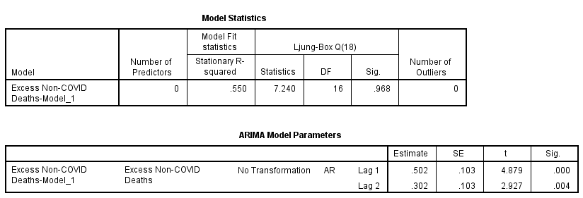
Excess non-COVID deaths turned out to be best modelled using an ARIMA(2,0,0) structure. In plain English this means this week’s value for excess death will be dependent on the previous week’s value and the week before that, this being what that number ‘2’ means. In gibberish we’re looking at an autoregressive component (AR) of order p=2. Lovers of ancient Greek will note that auto means ‘self’, so this can be translated as self-regression; that is, the data series looks back on itself for two weekly periods. And that’s it, there being nothing else to consider ‘coz of those zeroes. Philosophically speaking excess non-COVID death is a ‘memory’ and a short one at that, which is fascinating for this points to real world mechanisms of death that possess inertia, like a run of flu for instance or a run of freezing weather (hypothermia), or a spate of road accidents due to fog and ice. Herewith the model in the nude:

Thus, if we take 0.502 of last week’s value and add 0.302 of the value for the week previous we arrive at a prediction for this week’s value for excess non-COVID death. Though incredibly simplistic this two parameter model manages to scrape a most respectable stationary r-square¹ of 0.550. In plain English it does a good job. What will mangle minds here is that we are using the time series for excess non-COVID death to predict future values of itself (hence the 'auto' bit).

If that sounds a bit Dr Who (or even Star Trek) then consider a swinging pendulum that moves to and fro with regularity. After watching a few swings you’ll be able to predict where the swing is going next with relative ease - it’s the same with excess non-COVID death.

Stage 2: Case Detection Rate Model

Right then, a bit of nudity is in order:

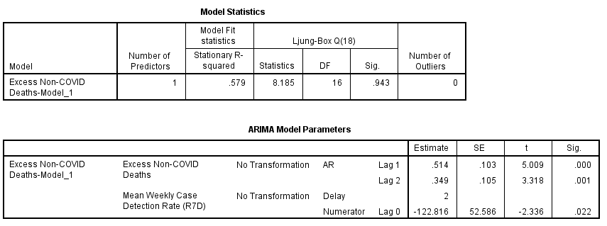
‘Elo, ‘elo, ‘elo, wot’s all this, then? It transpires that at a delay value of 2 weeks, my series for CDR crops up as a statistically significant predictor for excess non-COVID death (p=0.022), and in doing so it hikes our stationary r-square to 0.579. In plain English this means the series for excess non-COVID death, along with the series for CDR, explains 57.9% of the variation we see in excess non-COVID death. Has anybody noticed the negative coefficient - we’ll get to the bottom of this wacko a little later!

Now that’s an interesting brace of findings. ARIMA has decided 2 weeks is the optimum delay from detection to death in the modelling of excess death. It has also determined that CDR is correlated over time with excess non-COVID death even though these are supposed to be non-COVID deaths. This confirms my suspicion that death certification for COVID cases is a murky affair!

So what about that coefficient of determination? This pops out the pot at r-square = 0.051. In plain English this means 5.1% of the variation we see in excess non-COVID death can be explained by variation in the case detection rate at a lag of 2 weeks, this being a proxy for disease prevalence. One way we could look at this is to declare that around 5% of death certificates were not as they should have been.

Stage 3: Combined Dosing Model

Now for the star turn, starting with some nudity:

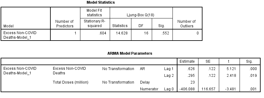
Well there you go! The time series for combined daily doses yields a highly statistically significant result (p=0.001) when set to a delay of 23 weeks, this being the very best model I can squeeze out. Right there in the nude for all to see is what appears to be confirmation of Steve Kirsch’s 5-month finding. So, now look at the stationary r-square value which has risen to 0.604; doses are doing a smashing job! But check out the negative coefficient. H’mmmm…..

So what about that there coefficient of determination? This pops out of the cooking pot at r-square = 0.299. In plain English this means 29.9% of the variation we see in excess non-COVID death can be explained by variation in combined daily dosing at a lag of 23 weeks. One way we could look at this is to declare that around 30% of excess non-COVID deaths are somehow inextricably linked to prior vaccination activity.

Stage 4: Case Detection Rate & Combined Dosing Model

We now go belt and braces and combine the two models with their respective delays set at 2 weeks and 23 weeks. In doing so we account for those erroneously coded deaths and get a better handle on what vaccination has likely been doing. Herewith the twin tables:

The first thing to note here is that CDR has come a cropper, displaying a non-significant p-value of p=0.063, though this is being picky since 90% confidence intervals are also bandied about in medical science, things not being so precise and all that. Let us then declare this as borderline and a poor cousin to combined dosing which gets top billing at p<0.001 at a lag of 23 weeks. We may note that the stationary r-square has now crept up to 0.625, this marking a slight improvement in the model fit.

The coefficient of determination drops out of the grill pan at r-square = 0.335. In plain English this means 33.5% of the variation we see in excess non-COVID death can be explained by variation in combined daily dosing at a lag of 23 weeks together with case detection rate at a lag of 2 weeks. Call that 34% and we have just over a third of the variation in excess deaths being explained by this combi boiler.

The Pudding

There is always a pudding in my club and here it is:

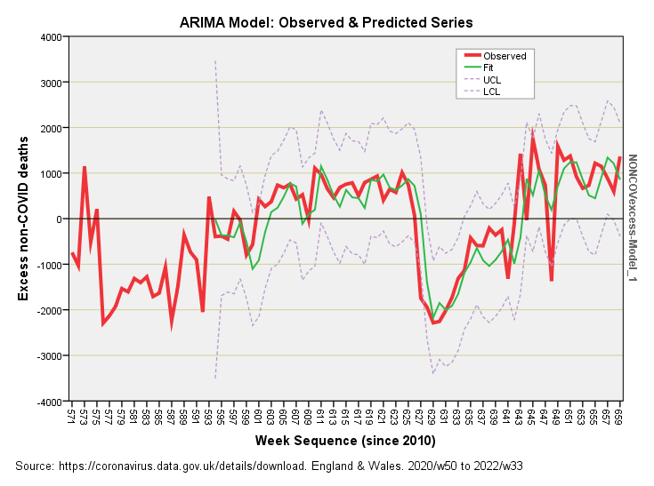
How about them apples? Some eagle-eyed types will ask why the green line doesn’t start at the beginning and this is because of that 23 week delay we dialled into the combined model. Note how the observed series bobs about within the 95% confidence intervals for the combi model, scraping them at a couple of points and bursting through at week sequence 648 (a.k.a. 2022/w22 a.k.a. w/e 3 Jun 2022).

Coffee & Cogitation

I hope folk supporting me financially have enjoyed this little adventure with ARIMA intervention analysis, it being a classic technique that has been used for all manner of serious work from evaluation of seat belt laws to forecasts of GNP to air traffic planning to crime rate assessment to fossil fuel consumption. What this work has done is convince me that something peculiar is afoot and we can’t go blaming viral variants.

The thing about excess death is that a surge across the population of England & Wales of this magnitude hasn’t come about by chance. Something very real is driving it. That something must have national impact and our list of suspects includes: COVID, long-COVID, lockdown and vaccines. We’ve seen that COVID plays a minor role and we may presume long-COVID and the impact of disastrous lockdown polices must also play a role.

At this point I suggest we retire to the lounge for stiff brandies or a decent cuppa, in which case it’s…

Kettle On!

1. Not to be confused with plain-old r-square which is useless in this context. Geeks might want to go right back to the source, this being: Harvey, A.C. (1989) Forecasting, Structural Time Series and the Kalman Filter. Cambridge: Cambridge University Press.